
The beauty of R is its versatility and of course the community 💜 you can use R for literally anything (I use blogdown to set up and maintain my website, xaringan to create slide decks, Shiny to build web applications, ….). All these great tools build upon one “little” (or not so little) thing: functions!
💡 What are functions?
A function is an inherent code block that performs a specific task, such as calculating a sum. And that’s exactly what we are doing now 😊
👩🏼💻 How to write them?
In R, functions can be as simple as this:
name_of_the_function <- function(arguments) {
  function_content
}
You give your function a name (name_of_the_function), define some arguments (arguments), and put some content in the function. Here you define how the function should proceed with the input (function_content).
Let’s use a simple example - a function that calculates the sum:
make_sum <- function(a, b) {
  c <- a + b
  return(c)
}
You have the name of your function (make_sum), two arguments (a and b), and the operation inside the function (calculating the sum, storing it in c, and returning c). You theoretically don’t have to use the return statement here because the function will implicitly return the last object created but I prefer to be more explicit and to have more control (and understanding) of what my function does 🤓
When I write functions, I usually have a more or less working code in my head or a script, copy-paste it into the function environment and let it run (it comes, of course, with a lot of debugging and problem-solving time).
Writing more complex functions
Writing functions is like a flower that blooms - you start simple and add more and more parts to it (like petals) 🌸 To explain what I mean, I will use the function overview_na from the {overviewR} package. The function allows you to plot the share of missing values in your data set.
When writing a function, I usually first set up a simple architecture of the function. The code snippet shows such an example: The function takes the data object, 1) uses an apply function to get the number of NAs by column, 2) converts the result to a data frame object and 3) plots it with {ggplot2}.
# How to plot NAs in your data 🕵
# # Based on `overview_na` from {overviewR}:
# https://github.com/cosimameyer/overviewR/blob/master/R/overview_na.R


overview_na <-
  function(dat
  ) {
    # Generate necessary variables ----------------------------------------
    # Calculate the number of NAs per column
    na_count <-
      sapply(dat, function(y)
        sum(length(which(is.na(
          y
        )))))
    # Convert it to the a data.frame
    dat_frame <- data.frame(na_count)
    # Add rownames_to_columns
    dat_frame <-
      tibble::rownames_to_column(dat_frame, var = "variable")

    # Plot vour visualization ---------------------------------------------
    # Create a aaplot2 with vour normal wav to create a ggplot2
    plot <- ggplot2::ggplot(data = dat_ frame)
    ggplot2::geom_col(ggplotz::aes(y = reorder(variable,-na_count),
                                   x = na_count))

    # Return the plot
    return(plot)
  }
The function already works but you can tweak it further (and that’s what I mean with the blooming and flower petal part 🌸 - it’s like adding another piece of beauty to it). You can now, for instance, allow the user to manually define the label of your x axis by adding an “xlabel” argument to your function (you are generally free to select an argument name that you want). The new parts are in-between the sparkles ✨
# How to plot NAs in your data 🕵
# # Based on `overview_na` from {overviewR}:
# https://github.com/cosimameyer/overviewR/blob/master/R/overview_na.R


overview_na <-
  function(dat,
           # ✨✨✨✨✨✨✨✨✨✨✨✨✨✨✨✨✨✨✨✨✨✨✨✨
           # Add a manual xlabel for your plot ✨
           # The default will be "Showing your NAs" but
           # you can change it and also add a different label
           xlabel = "Showing your NAs"
           # ✨✨✨✨✨✨✨✨✨✨✨✨✨✨✨✨✨✨✨✨✨✨✨✨
  ) {
    # Generate necessary variables ----------------------------------------
    # Calculate the number of NAs per column
    na_count <-
      sapply(dat, function(y)
        sum(length(which(is.na(
          y
        )))))
    # Convert it to the a data.frame
    dat_frame <- data.frame(na_count)
    # Add rownames_to_columns
    dat_frame <-
      tibble::rownames_to_column(dat_frame, var = "variable")

    # Plot vour visualization ---------------------------------------------
    # Create a aaplot2 with vour normal wav to create a ggplot2
    plot <- ggplot2::ggplot(data = dat_ frame)
    ggplot2::geom_col(ggplotz::aes(y = reorder(variable,-na_count),
                                   x = na_count)) +
      # ✨✨✨✨✨✨✨✨✨✨✨✨✨✨✨✨✨✨✨✨✨✨✨✨
      ggplot2::xlab(xlabel)
      # ✨✨✨✨✨✨✨✨✨✨✨✨✨✨✨✨✨✨✨✨✨✨✨✨
    # Return the plot
    return(plot)
  }
Or use a pre-defined theme 💅 You can add the theme to your function but you can also put it in extra function as I did (makes debugging so much better (and your code cleaner 👍, the theme that we use in {overviewR} is here)).
# How to plot NAs in your data 🕵
# # Based on `overview_na` from {overviewR}:
# https://github.com/cosimameyer/overviewR/blob/master/R/overview_na.R


overview_na <-
  function(dat,
           xlabel = "Showing your NAs") {
    # ✨✨✨✨✨✨✨✨✨✨✨✨✨✨✨✨✨✨✨✨✨✨✨✨
    # Set theme -----------------------------------------------------------
    # Create a theme for the plot
    # The theme is created here:
    # https://bit.ly/theme_na_plot
    # It is a basic ggplot2::theme
    theme_plot <- theme_na_plot()
    # ✨✨✨✨✨✨✨✨✨✨✨✨✨✨✨✨✨✨✨✨✨✨✨✨

    # Generate necessary variables ----------------------------------------
    # Calculate the number of NAs per column
    na_count <-
      sapply(dat, function(y)
        sum(length(which(is.na(
          y
        )))))
    # Convert it to the a data.frame
    dat_frame <- data.frame(na_count)
    # Add rownames_to_columns
    dat_frame <-
      tibble::rownames_to_column(dat_frame, var = "variable")

    # Plot vour visualization ---------------------------------------------
    # Create a aaplot2 with vour normal wav to create a ggplot2
    plot <- ggplot2::ggplot(data = dat_ frame)
    ggplot2::geom_col(ggplotz::aes(y = reorder(variable, -na_count),
                                   x = na_count)) +
      ggplot2::xlab(xlabel)

    # Return the plot
    return(plot)
  }
✨ Best practices when writing functions
Let’s dig into best practices when it comes to function writing. This list contains a loose collections of tips and tricks that are not ranked in a particular order:
- Use curly brackets - it makes it easier to read and work with your functions.

Alternative text
Good practice vs. not-so-good practice
##Good practice
make_sum <- function(a, b) {
  c <- a + b
  return(c)
}

##Not so good practice
make_sum <- function(a, b)  a + c
- Use meaningful names for your functions. It’s good to use verbs for functions.
- Use also meaningful names for your arguments. It’s common practice to use nouns to name the arguments.
- Once your function gets longer, write assertions, warnings, and stops. This allows you (and the user) to prevent something goes wrong and/or to learn immediately when something goes wrong (and is also helpful for future debugging - we will talk about this in the next post 🎊 If you’re curious, here’s a Twitter thread that I wrote about it)
- If your function is too long, refactor it and build multiple sub-functions. Each function should do one thing at a time. This also makes your debugging life much easier.
- While it’s not necessary, I prefer to use an explicit
return(...)statement at the end of my function. By default, your function will return your last generated output. Returning it explicitly, however, allows you more control over your function (at least that’s how I feel about it and why I do it) - If you have a construct of functions, consider putting them into a package (that’s also what we’ll learn 😊)
- If you package your functions, create one R file for each function and name the R file the same way as your function.
For more tips and tricks, also have a look at Hadley Wickham’s and Garett Grolemund’s excellent book “R for Data Science”.
If you want to quickly look up what this blog post tells you about writing functions, here’s a summary (also as 📄PDF for you to download here):
Alternative text
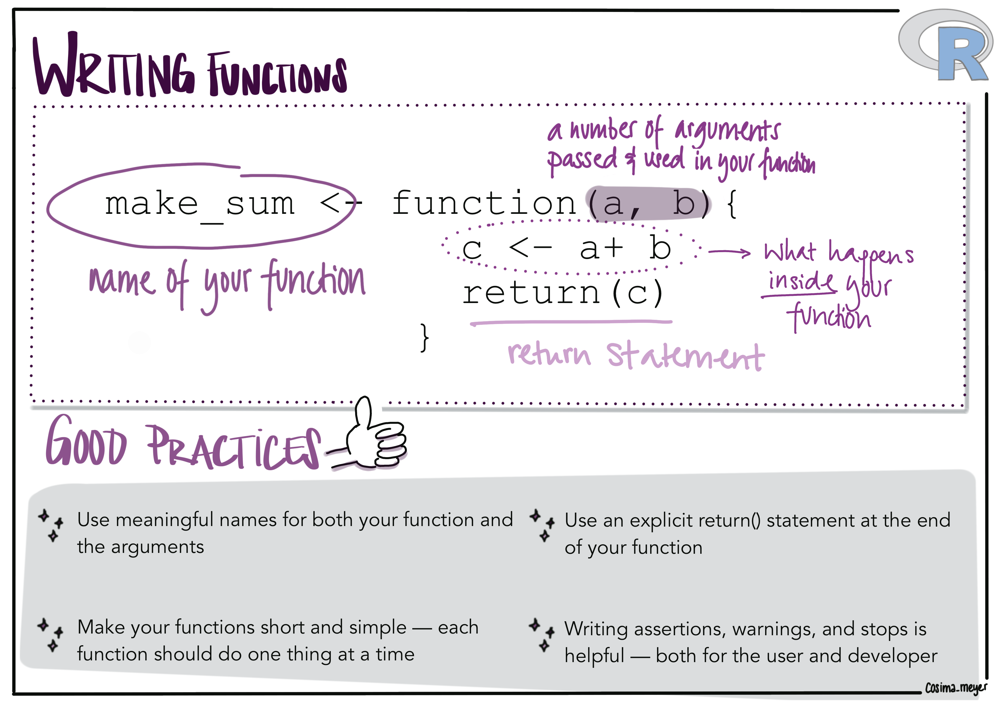
Image showing how a general function in R looks like (a function has arguments, a function statement, and usually a return function). Good practices when writing functions are:
- Use meaningful names for your functions. It’s good to use verbs for functions
- Make your function short and simple - each function should do one thing at a time
- Use an explicit return statement
- Writing assertions, warnings and stops is helpful